back to home

by Justin Chappell 12/30/2024

Rendering Math Fundamentals

Introduction

Have you ever wondered how computers display 3D graphics? How can we depict 3D environment on a ‘2D’ screen? In this blog I will put forward the basic math required to accomplish this. My intention is for this blog to be more of a reference rather than spending too much time on specifics. For more in-depth coverage of this topic as well as helpful resources I have provided a bunch of links at the end of the blog if you’re interested.

What 3D graphics rasterisers do is quite simple, they project geometry defined in 3D space onto a 2D rectangle (your screen).

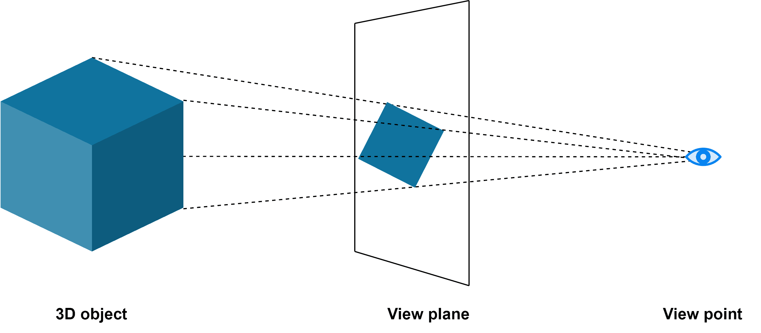
Here is the equation that computes the projection of 3D geometry onto the view plane.

$\vec{v_p}\prime=PVM\vec{v_p}$

On the LHS we have our final vertex position (projected to our view rectangle), and on the RHS we see the perspective, view and model matrices multiplied against the vertex positions of some defined geometry in 3D space.

1. Perspective ($P$): As the name suggest this matrix defines the what objects look like at different distances from our view. Effectively defining what is called the view frustrum. Objects closer to the origin of our view will appear bigger or smaller depending on the type of frustrum created. This gives us the ability to perceive depth.

There are plenty of different perspective matrices at our dispense, but by far the most common one used in 3D games/graphics is the perspective projection matrix.

2. View ($V$): We can think of the view matrix as a sort of camera. Different from cameras in real life, this camera has less to do with light sensors and more to do with where we are and what are we looking.

3. Model ($M$): If we wish to either scale, rotate or translate and object in a 3D scene we can do that through the model matrix. This matrix defines the scale rotation and location of an object in our 3D scene.

Now with that brief overview of what we are aiming towards, I will now spend the rest of this blog going through the mathematics required to implement such a renderer.

Vectors

Vectors describe different things depending on their context. They are useful in grouping similar information into a neat package. In graphics vectors can be used to describe positions of vertices (xyz), colours (rgb), quaternions (wxyz). For most cases the values are float/reals, but sometimes it may come in handy to have integer based components or other types.

Operations

ADDITION: $\vec{a}+\vec{b}=\begin{bmatrix}x\\y\\z\end{bmatrix}+\begin{bmatrix}x\\y\\z\end{bmatrix}=\begin{bmatrix}2x\\2y\\2z\end{bmatrix}\\$ Add two vectors component-wise.

SUBTRACT: $\vec{a}-\vec{b}=\begin{bmatrix}x\\y\\z\end{bmatrix}-\begin{bmatrix}x\\y\\z\end{bmatrix}=\begin{bmatrix}0\\0\\0\end{bmatrix}\\$ Subtract two vectors component-wise.

MULTIPLY: $\vec{a}\vec{b}=\begin{bmatrix}x\\y\\z\end{bmatrix}\begin{bmatrix}x\\y\\z\end{bmatrix}=\begin{bmatrix}x^2\\y^2\\z^2\end{bmatrix}\\$ Multiply two vectors component-wise.

DOT: $\vec{a}\cdot\vec{b}=\vec{a}\cdot\vec{b}=\begin{bmatrix}x\\y\\z\end{bmatrix}\cdot\begin{bmatrix}x\\y\\z\end{bmatrix}=a_0b_0+a_0b_0+a_1b_1\\$ The inner product of two same length vectors results in a scalar value showing the similarity in pointing direction of the to vectors.

CROSS: $\vec{a}\times\vec{b}=\begin{bmatrix}a_1b_2 - a_2b_1\\-a_0b_2 - a_2b_0\\a_0b_1 - a_1b_0\end{bmatrix}\\$ Produces an orthogonal vector to both vectors.

MAGNITUDE: $|\vec{a}|=\sqrt{a_x^2+a_y^2+a_z^2}\\$ Vector length.

UNIT: $\hat{a}=\frac{\vec{a}}{|\vec{a}|}\\$ Unit length vector (length of 1).

Matrices

Similarly to vectors, the contents of a matrix depend on the context that you use them. In most of 3D graphics we will be dealing with 4x4 (float/real values) matrices. Graphics APIs like OpenGL don’t care if your matrices are row or column major; however, whatever major you major in :) keep it consistent. Furthermore, if you are in the wrong major just transpose the matrix in question.

Operations

IDENTITY: $I=\begin{bmatrix} 1 & 0 & 0 & 0\\ 0 & 1 & 0 & 0\\ 0 & 0 & 1 & 0\\ 0 & 0 & 0 & 1 \end{bmatrix}\\$ Must be a square matrix, unique property that if you multiply some other matrices of the same size by the identity matrix the other matrix will be the result.

ADDITION: Similar to vectors, do component-wise addition

SUBTRACT: Similar to vectors, do component-wise subtraction

MULTIPLY: $AB=\begin{bmatrix} a & b\\ c & d \end{bmatrix} \begin{bmatrix} e & f\\ g & h \end{bmatrix}= \begin{bmatrix} ae + bg & af + bh\\ ce + dg & cf + dh\\ \end{bmatrix}\\$ Same process for larger matrices.

TRANSPOSE: $A= \begin{bmatrix} a & b\\ c & d \end{bmatrix},\\ A^T=\begin{bmatrix} a & c\\ b & d \end{bmatrix}\\$ Essentially reflecting the matrix along the leading diagonal. Same process for larger matrices.

Matrix Transformations

In this section I will cover the basic transformation matrices required to scale, rotate and translate geometry. These matrices are fundamental for creating a model matrix as well as manipulating the view (camera) matrix.

Scale

$S=\begin{bmatrix} S_x & 0 & 0 & 0\\ 0 & S_y & 0 & 0\\ 0 & 0 & S_z & 0\\ 0 & 0 & 0 & 0\\ \end{bmatrix}$

Translation

$T=\begin{bmatrix} 0 & 0 & 0 & T_x\\ 0 & 0 & 0 & T_y\\ 0 & 0 & 0 & T_z\\ 0 & 0 & 0 & 0\\ \end{bmatrix}$

Rotation

I will only cover Euler rotations here; however, there are more efficient ways to calculate the rotation matrix. Namely using quaternions. I will cover quaternions in a separate blog eventually.

For each axis we need to define a 3x3 rotation matrix.

The final rotation matrix is formed by multiplying in order of yaw pitch and roll $R=R_z(\theta_z)R_y(\theta_y)R_x(\theta_x)$.

$\theta$ is in radians.

$R_x(\theta)=$$\begin{bmatrix} 1 & 0 & 0\\ 0 & cos{\theta} & -sin{\theta}\\ 0 & sin{\theta} & cos{\theta}\\ \end{bmatrix}\\$

$R_y(\theta)=$$\begin{bmatrix} cos{\theta} & 0 & sin{\theta}\\ 0 & 1 & 0\\ -sin{\theta} & 0 & cos{\theta}\\ \end{bmatrix}\\$

$R_z(\theta)=$$\begin{bmatrix} cos{\theta} & -sin{\theta} & 0\\ sin{\theta} & cos{\theta} & 0\\ 0 & 0 & 1\\ \end{bmatrix}$

In practice the rotation matrix is a 4x4 matrix (just zero out the new row and column). This enables the multiplication of this matrix against the scale and translation matrix to form the model matrix $M$.

The order of this multiplication for the model matrix is:

$M=SRT$

Special Matrices

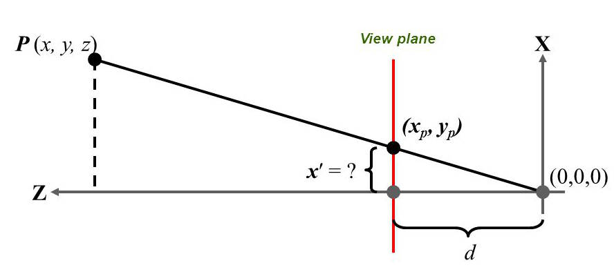
Perspective

$m00=\frac{1}{aspect\cdot\tan{(\theta_{fov}/2)}}\\$ $m11=\frac{1}{\tan{(\theta_{fov}/2)}}\\$ $m22=-\frac{far_z+near_z}{far_z-near_z}\\$ $m23=-\frac{2 far_z near_z}{far_z-near_z}\\$ $m32=-1\\$ $P=\begin{bmatrix} m00 & 0 & 0 & 0\\ 0 & m11 & 0 & 0\\ 0 & 0 & m22 & m23\\ 0 & 0 & m32 & 0 \end{bmatrix}\\$

aspect: Desired aspect ratio for the geometry to be rendered at.

$\theta_{fov}$: Field of view in radians.

$far_z$: Far clipping plane.

$near_z$: Near clipping plane.

View

$V=\begin{bmatrix} L_x & L_y & L_z & P_x\\ U_x & U_y & U_z & P_x\\ R_x & R_y & R_z & P_x\\ 0 & 0 & 0 & 1 \end{bmatrix}$

$L$: Left of the view (Camera).

$U$: Up of the view (Camera).

$R$: Right of the view (Camera).

$P$: View (Camera) position.

Helpful Resources

• Linear Algebra Done Right (Text Book)
• MIT Linear Algebra Course (Course)
• Model View Projection (ARTICLE)
• Essence of linear algebra (Video Playlist)
• Learn OpenGL (Tutorial)
• Learn Computer Graphics Using WebGL (Tutorial)